August 27, 2021
Create spatial square/hexagon grids and count points inside in R with sf
Generate Tessellation and Summarise Within, but in R
3175 words | 14-min read |
TL;DR
This article demonstrate and explains how to use the sf package to
complete the following two tasks:
- Create a custom tessellation grid (square cells or hexagon cells)
- Count the number of points within each cell
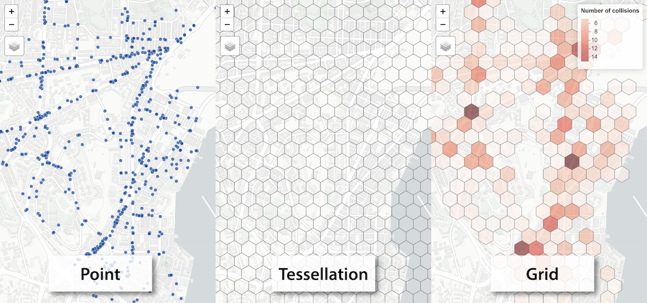
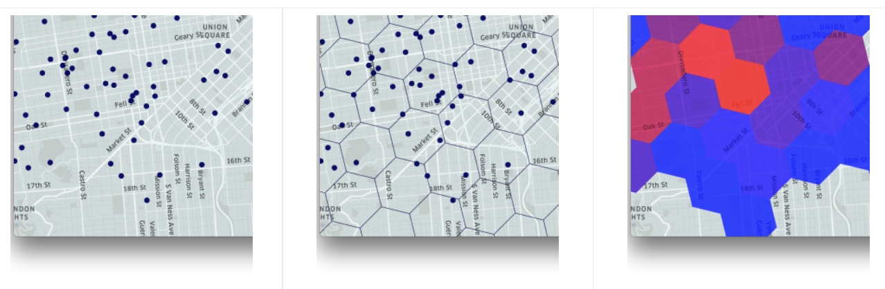
Spatial grids are commonly used in spatial analysis. The core concept is to divide the study of area into equal-size, regular polygons that could tessellate the whole study area. After that, a variable is summarised within each polygon. Alternatively speaking, the process is to “slice the study area into subunits over which we summarize a spatial variable” (quoting from Matt Strimas-Mackey’s article).
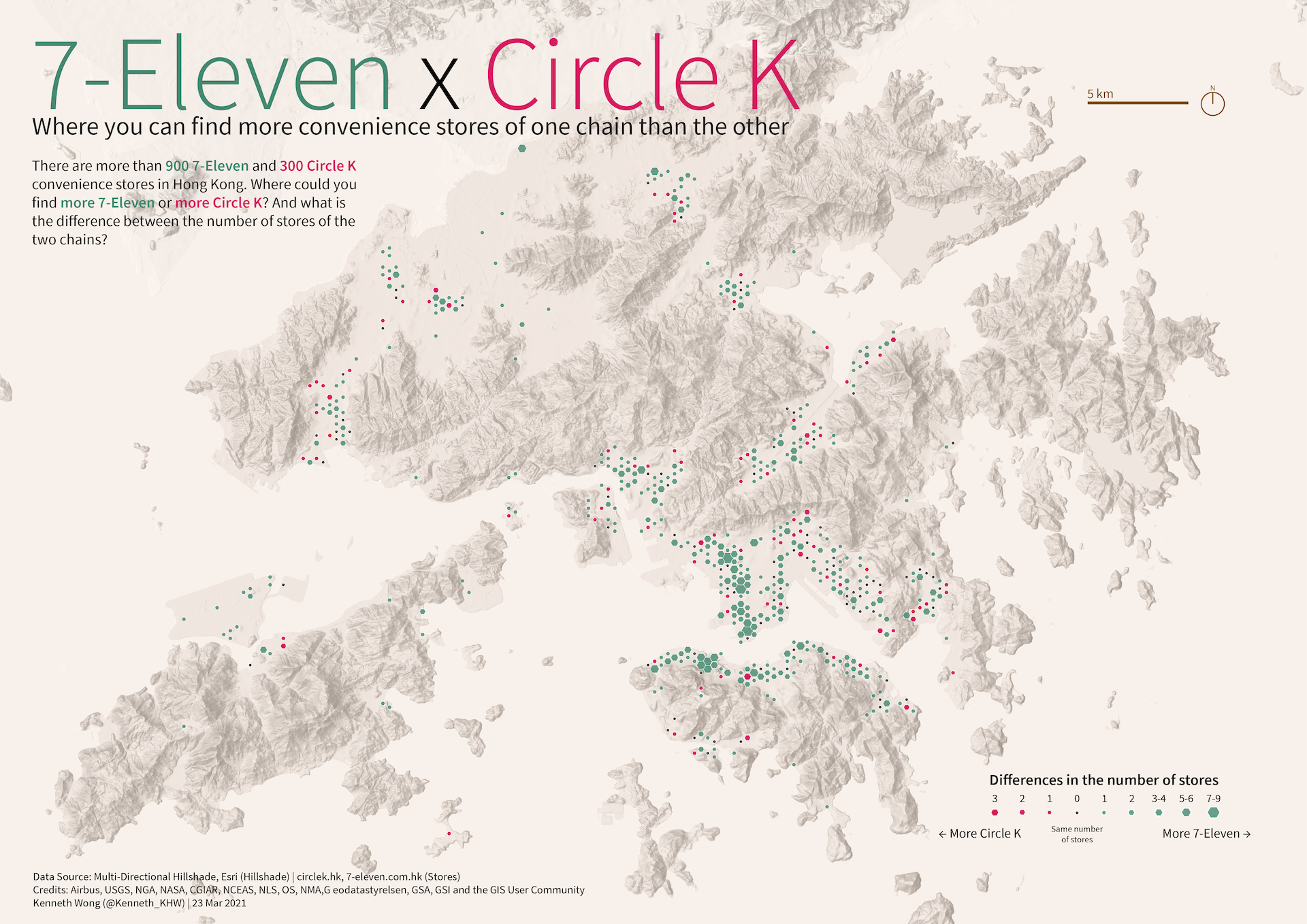
I frequently apply this method for my map-making project. I have a hexagonal grid data of land in Hong Kong for me to summarise variables including number of convenience stores, percentage of built-up area and number of ubiquitous urban facilities.
I usually use ArcGIS Pro or QGIS to do both “create tessellation” and “summarise variable” task. This time, I am going to replicate both tasks using R.
Setup
library(hkdatasets)
library(sf)
library(dplyr)
library(mapview)
library(tmap)
Get sample point data
In this example, I am using the hk_accidents dataset, a dataset of traffic collisions of Hong Kong from 2014 to 2019, from the hkdatasets package (available in CRAN and GitHub) The data is in already in tidy format. Just two additional steps are required before making grids:
- Subset the data (the whole dataset has more than 95,000 rows! Probably too large for demonstration purposes)
- Converting the data from data.frame to
sfobject
# traffic collision of Hong Kong from 2014 to 2019
hk_accidents = hkdatasets::download_data("hk_accidents")

# collisions in Kowloon City District, 2017
test_data = subset(hk_accidents, District_Council_District == "KC" & Year == 2017)

# turn it to sf object
test_points = test_data %>%
  # lng/lat value are missing in some records
  filter(!is.na(Grid_E) & !is.na(Grid_N)) %>%
  st_as_sf(coords = c("Grid_E", "Grid_N"), crs = 2326, remove = FALSE)
And these are the traffic collisions in the Kowloon City District of Hong Kong in 2017.
mapview_test_points = mapview(test_points, cex = 3, alpha = .5, popup = NULL)

mapview_test_points
Square grid (fishnet)
Square grids, sometimes called fishnet, are more common method of tessellation because of its resemblances to orthodox square raster grids in GIS.
We will first create a grid which the extent equals to the bounding box of the selected points.
area_fishnet_grid = st_make_grid(test_points, c(150, 150), what = "polygons", square = TRUE)

# To sf and add grid ID
fishnet_grid_sf = st_sf(area_fishnet_grid) %>%
  # add grid ID
  mutate(grid_id = 1:length(lengths(area_fishnet_grid)))
Then, count the number of points in each grid.
# count number of points in each grid
# https://gis.stackexchange.com/questions/323698/counting-points-in-polygons-with-sf-package-of-r
fishnet_grid_sf$n_colli = lengths(st_intersects(fishnet_grid_sf, test_points))

# remove grid without value of 0 (i.e. no points in side that grid)
fishnet_count = filter(fishnet_grid_sf, n_colli > 0)
And then we have it! To check the result, plot the grid into a
interactive thematic map with tmap.
tmap_mode("view")

map_fishnet = tm_shape(fishnet_count) +
  tm_fill(
    col = "n_colli",
    palette = "Reds",
    style = "cont",
    title = "Number of collisions",
    id = "grid_id",
    showNA = FALSE,
    alpha = 0.5,
    popup.vars = c(
      "Number of collisions: " = "n_colli"
    ),
    popup.format = list(
      n_colli = list(format = "f", digits = 0)
    )
  ) +
  tm_borders(col = "grey40", lwd = 0.7)

map_fishnet
Hexagon grid (honeycomb)
Hexagon (honeycomb) grids is another popular choice of grids. I find hexagonal girds usually more visually appealing and use them in most of my mapping projects.
The steps of making a hexagonal grid and summarise the points within
each grid is 99% the same from the square grid one shown above. The only
difference is changing the argument from square = TRUE to
square = FALSE in st_make_grid.
area_honeycomb_grid = st_make_grid(test_points, c(150, 150), what = "polygons", square = FALSE)

# To sf and add grid ID
honeycomb_grid_sf = st_sf(area_honeycomb_grid) %>%
  # add grid ID
  mutate(grid_id = 1:length(lengths(area_honeycomb_grid)))

# count number of points in each grid
# https://gis.stackexchange.com/questions/323698/counting-points-in-polygons-with-sf-package-of-r
honeycomb_grid_sf$n_colli = lengths(st_intersects(honeycomb_grid_sf, test_points))

# remove grid without value of 0 (i.e. no points in side that grid)
honeycomb_count = filter(honeycomb_grid_sf, n_colli > 0)
tmap_mode("view")

map_honeycomb = tm_shape(honeycomb_count) +
  tm_fill(
    col = "n_colli",
    palette = "Reds",
    style = "cont",
    title = "Number of collisions",
    id = "grid_id",
    showNA = FALSE,
    alpha = 0.6,
    popup.vars = c(
      "Number of collisions: " = "n_colli"
    ),
    popup.format = list(
      n_colli = list(format = "f", digits = 0)
    )
  ) +
  tm_borders(col = "grey40", lwd = 0.7)

map_honeycomb
How does the code work?
Create tessellation
The tessellation is created using the st_make_grid function.
test_pointsis the input spatial data. The function will define the bounding box (processing extent in ArcGIS sense) of the tessellation.c(150, 150)is the cell size, in the unit the crs of the spatial data is using. The default option splits the bounding box into 100 grids, 10 rows x 10 columns layout. I prefer stating the cell size, since the sense of distance could differs according to the spatial variable you are analysing.- square argument indicates whether you are a square grid (TRUE) or hexagon grid (FALSE)
Caveat: The cell size is in the same unit to the projected coordinate system (pcs) of the spatial data (in this case, meters). If the values are too small, R will produce a disastrous amount of grids that could make your laptop crash.
Diego HH provides a great summary and experiments with the
st_make_grid function in his Beautiful Maps with R (I): Fishnets,
Honeycombs and Pixels
article. Actually, I referred to his code so many times when trying to
create various grids!
area_honeycomb_grid = st_make_grid(test_points, c(150, 150), what = "polygons", square = FALSE)
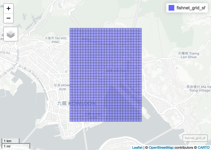
Here is what the basic tessellation looks like.
mapview(fishnet_grid_sf)
Adding Grid ID
st_make_grid returns a sfc_POLYGON object. st_sf is used to
convert to sf object for easier handling.
Adding an unique ID to each cell could help identify the cells when
further analysis are needed. length(lengths(area_honeycomb_grid))
returns the total number of cells created. Then we could create a
columns of grid_id labelling each cell, from 1 to largest.
# To sf and add grid ID
fishnet_grid_sf = st_sf(area_fishnet_grid) %>%
  # add grid ID
  mutate(grid_id = 1:length(lengths(area_fishnet_grid)))
Count number of points in each grid
The tools here is st_intersects, when using polygon (here, grid)
as the first input and point (here, traffic collision location) as
the second input, st_intersects will return a list of which points are
lying inside each grid.
st_intersects(fishnet_grid_sf, test_points)
## Sparse geometry binary predicate list of length 945, where the
## predicate was `intersects'
## first 10 elements:
##  1: (empty)
##  2: (empty)
##  3: (empty)
##  4: (empty)
##  5: (empty)
##  6: (empty)
##  7: (empty)
##  8: (empty)
##  9: 104, 253
##  10: 632
But we are not much interested in which point lies in which grid. The
things need to know is how many points are within each grid. lengths
will return the number of each element of the list.
lengths(st_intersects(fishnet_grid_sf, test_points))
##   [1]  0  0  0  0  0  0  0  0  2  1  1  1  0  0  0  0  0  0  0  0  0  0  0  0  0
##  [26]  0  0  0  0  0  0  0  0  0  2  2  0  3  0  0  1  0  0  0  0  0  0  0  0  0
##  [51]  0  0  0  0  0  0  0  0  0  0  0  2  0  2  2  1  1  1  0  0  0  0  0  0  0
##  [76]  0  0  0  0  0  0  0  0  0  0  0  0  4  5  7 10  0  0  3  0  0  0  0  0  0
## [101]  0  0  0  0  0  0  0  0  0  0  0  0  0  2  9  4  7  5  1  3  1  0  0  0  0
## [126]  0  0  0  0  0  0  0  0  0  2  0  0  0  0  0  0  0 24  3  5  0  0  0  0  0
## [151]  0  0  0  0  0  0  0  0  0  0  0  1  0  0  0  0  3  0  1  2  7  5  0  6  0
## [176]  0  0  0  0  0  0  0  0  0  0  0  0  0  1  0  0  2  3  0  0  2  0  9  7  7
## [201]  4  0  0  0  0  0  0  0  0  0  0  0  0  0  0  0  0  0  1  1  0  0  2  0  0
## [226]  7  1  1  0  0  0  0  0  0  0  0  0  0  0  1  0  0  0  0  0  2  3  0  3  0
## [251]  0  0  6  5  2  0  1  0  0  0  0  0  0  0  0  2  0  0  0  0  0  0  0  1  4
## [276]  6  0  0  0  5 10  7  2  2  0  0  0  0  0  0  0  0  0  0  1  0  0  2  2  3
## [301] 13  8  0  0  0  0  2 12  3  5  3  1  0  0  0  0  0  0  0  0  0  0  0  0  2
## [326] 11  1  0  0  2  1  0  1  5  5  2  3  8  2  0  0  0  0  0  0  0  0  0  0  0
## [351]  0  8  3  4  5  1  0  2  0  3 13  0  1  2  4  1  0  0  0  0  0  0  0  0  0
## [376]  0  0  0  0  0  0 24  3  0  0  0  2  3  5  6  6  2  2  0  0  0  0  0  0  0
## [401]  0  0  0  0  0  0  0  0  1  1  2  2  0  0  1  7  2  4  0  1  0  0  0  0  0
## [426]  0  0  0  0  0  0  0  4  5  0  5  0  0  0  4 11  0 10  1  0  1  1  0  0  0
## [451]  0  1  0  0  0  0  0  0  0  2  3  4  9  4  4  3  0  0  8  2  5  0  0  0  0
## [476]  0  0  0  0  0  0  0  0  0  0  0  0  1  1  6  2  2  0  5  5 13  7 20  3  0
## [501]  0  0  1  0  0  0  1  0  0  0  0  0  0  0  0  1  5  0  0  2  2  1  9  5  8
## [526]  7  6  0  0  0  0  0  0  0  0  0  0  0  0  0  0  0  0  5  1  2  1  0  0  3
## [551]  1  4  0  4  2  0  0  0  0  0  0  0  0  0  0  0  0  0  0  0  4  1  0  0  0
## [576]  0  8  1  1  1  0  0  1  0  0  0  0  1  2  0  0  0  0  0  0  0  0 11  0  3
## [601]  0  0  0  0  0  0  0  0  0  0  2  0  1  0  0  0  0  0  0  0  0  0  0  0 10
## [626]  2  1  4  0  0  1  0  0  0  0  0  0  0  0  1  2  0  1  0  0  0  0  0  0  0
## [651]  0  0  1  0  0  0  0  0  0  0  0  0  0  0  0  0  0  4  5  0  0  0  0  0  0
## [676]  0  0  4  3  4  3  0  0  0  0  0  0  0  0  0  0  0  0  0  0  0  0  0  0  0
## [701]  0  0  0  0  0  2  4  1  0  0  1  0  0  0  0  0  0  0  0  0  0  0  0  0  0
## [726]  0  0  0  0  0  0  2  0 14  2  0  1  0  0  0  0  0  0  0  0  0  0  0  0  0
## [751]  0  0  0  0  0  0  1  6  0  1  3  0  0  1  0  0  0  0  0  0  0  0  0  0  0
## [776]  0  0  0  0  0  0  0  0  0  0  0  1  0  2  0  0  0  0  0  0  0  0  0  0  0
## [801]  0  0  0  0  0  0  0  0  0  0  0  0  1  5  3  1  7  2  0  0  0  0  0  0  0
## [826]  0  0  0  0  0  0  0  0  0  0  0  0  0  2  1  5  3  7  0  0  0  0  0  0  0
## [851]  0  0  0  0  0  0  0  0  0  0  0  0  0  0  0  0  0  0  0  2  0  0  0  0  0
## [876]  0  0  0  0  0  0  0  0  0  0  0  0  0  0  0  0  0  0  0  0  0  0  0  0  0
## [901]  0  0  0  0  0  0  0  0  0  0  0  0  0  0  0  0  0  0  0  0  0  0  1  0  0
## [926]  0  0  0  0  0  0  0  0  0  0  0  0  0  0  0  0  0  0  0  0
With this list of “count of points”, we could attach it back to the grid
sf object. The dataframe will have a new column named n_colli, storing
the number of points (collisions) in each cell.
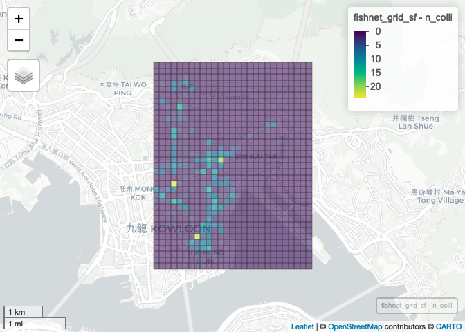
fishnet_grid_sf$n_colli = lengths(st_intersects(fishnet_grid_sf, test_points))
We would easily check the results by symbolising each grid according to the number of collisions.
mapview(fishnet_grid_sf, zcol = "n_colli")
Thanks Michael Sumner for providing the solution of counting points in polygon from this GIS StackExchange question.
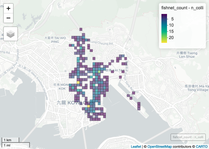
Remove grids with 0 values
Yet, there are some cells without any collision points inside. Showing them will be redundant and churns out the computer space, especially when the points tends to be clustered within some major areas. I tend to remove those cells with count of points equals to 0. That reduces the amount of information the reader have to understand.
fishnet_count = filter(fishnet_grid_sf, n_colli > 0)
mapview(fishnet_count, zcol = "n_colli")
And that’s how to create tessellation and count points in polygons using R.
How to do it in ArcGIS Pro & QGIS?
As a quick reference, here’s how I complete the same task in ArcGIS Pro and QGIS.
In ArcGIS Pro:
- Generate Tessellation
- Summarize Within or Spatial Join
- Filter out grids with 0 values using Select by attributes function
In QGIS:
- Use Create grid layer tool in MMQGIS Plugin
- Count points in polygon
- Check this post from GIS Lounge for detailed steps!
References
Beautiful Maps with R (I): Fishnets, Honeycombs and Pixels
Counting points in polygons with sf package of R? - GIS StackExchange
Spatial Modelling Tidbits: Honeycomb or Fishnets?
Session Info
sessioninfo::session_info()
Session Info
## ─ Session info ───────────────────────────────────────────────────────────────
##  setting  value
##  version  R version 4.1.0 (2021-05-18)
##  os       macOS Big Sur 10.16
##  system   x86_64, darwin17.0
##  ui       X11
##  language (EN)
##  collate  en_US.UTF-8
##  ctype    en_US.UTF-8
##  tz       Asia/Hong_Kong
##  date     2021-09-10
##
## ─ Packages ───────────────────────────────────────────────────────────────────
##  package           * version  date       lib source
##  abind               1.4-5    2016-07-21 [1] CRAN (R 4.1.0)
##  assertthat          0.2.1    2019-03-21 [1] CRAN (R 4.1.0)
##  base64enc           0.1-3    2015-07-28 [1] CRAN (R 4.1.0)
##  brew                1.0-6    2011-04-13 [1] CRAN (R 4.1.0)
##  callr               3.7.0    2021-04-20 [1] CRAN (R 4.1.0)
##  class               7.3-19   2021-05-03 [1] CRAN (R 4.1.0)
##  classInt            0.4-3    2020-04-07 [1] CRAN (R 4.1.0)
##  cli                 2.5.0    2021-04-26 [1] CRAN (R 4.1.0)
##  codetools           0.2-18   2020-11-04 [1] CRAN (R 4.1.0)
##  colorspace          2.0-1    2021-05-04 [1] CRAN (R 4.1.0)
##  crayon              1.4.1    2021-02-08 [1] CRAN (R 4.1.0)
##  crosstalk           1.1.1    2021-01-12 [1] CRAN (R 4.1.0)
##  data.table          1.14.0   2021-02-21 [1] CRAN (R 4.1.0)
##  DBI                 1.1.1    2021-01-15 [1] CRAN (R 4.1.0)
##  dichromat           2.0-0    2013-01-24 [1] CRAN (R 4.1.0)
##  digest              0.6.27   2020-10-24 [1] CRAN (R 4.1.0)
##  dplyr             * 1.0.7    2021-06-18 [1] CRAN (R 4.1.0)
##  e1071               1.7-7    2021-05-23 [1] CRAN (R 4.1.0)
##  ellipsis            0.3.2    2021-04-29 [1] CRAN (R 4.1.0)
##  evaluate            0.14     2019-05-28 [1] CRAN (R 4.1.0)
##  fansi               0.5.0    2021-05-25 [1] CRAN (R 4.1.0)
##  farver              2.1.0    2021-02-28 [1] CRAN (R 4.1.0)
##  fst                 0.9.4    2020-08-27 [1] CRAN (R 4.1.0)
##  generics            0.1.0    2020-10-31 [1] CRAN (R 4.1.0)
##  glue                1.4.2    2020-08-27 [1] CRAN (R 4.1.0)
##  highr               0.9      2021-04-16 [1] CRAN (R 4.1.0)
##  hkdatasets        * 1.0.0    2021-09-04 [1] CRAN (R 4.1.0)
##  htmltools           0.5.1.1  2021-01-22 [1] CRAN (R 4.1.0)
##  htmlwidgets         1.5.3    2020-12-10 [1] CRAN (R 4.1.0)
##  jsonlite            1.7.2    2020-12-09 [1] CRAN (R 4.1.0)
##  KernSmooth          2.23-20  2021-05-03 [1] CRAN (R 4.1.0)
##  knitr               1.33     2021-04-24 [1] CRAN (R 4.1.0)
##  lattice             0.20-44  2021-05-02 [1] CRAN (R 4.1.0)
##  leafem              0.1.6    2021-05-24 [1] CRAN (R 4.1.0)
##  leaflet             2.0.4.1  2021-01-07 [1] CRAN (R 4.1.0)
##  leaflet.providers   1.9.0    2019-11-09 [1] CRAN (R 4.1.0)
##  leafpop             0.1.0    2021-05-22 [1] CRAN (R 4.1.0)
##  leafsync            0.1.0    2019-03-05 [1] CRAN (R 4.1.0)
##  lifecycle           1.0.0    2021-02-15 [1] CRAN (R 4.1.0)
##  lwgeom              0.2-7    2021-07-28 [1] CRAN (R 4.1.0)
##  magrittr            2.0.1    2020-11-17 [1] CRAN (R 4.1.0)
##  mapview           * 2.10.0   2021-06-05 [1] CRAN (R 4.1.0)
##  munsell             0.5.0    2018-06-12 [1] CRAN (R 4.1.0)
##  pillar              1.6.1    2021-05-16 [1] CRAN (R 4.1.0)
##  pkgconfig           2.0.3    2019-09-22 [1] CRAN (R 4.1.0)
##  png                 0.1-7    2013-12-03 [1] CRAN (R 4.1.0)
##  processx            3.5.2    2021-04-30 [1] CRAN (R 4.1.0)
##  proxy               0.4-26   2021-06-07 [1] CRAN (R 4.1.0)
##  ps                  1.6.0    2021-02-28 [1] CRAN (R 4.1.0)
##  purrr               0.3.4    2020-04-17 [1] CRAN (R 4.1.0)
##  R6                  2.5.0    2020-10-28 [1] CRAN (R 4.1.0)
##  raster              3.4-13   2021-06-18 [1] CRAN (R 4.1.0)
##  RColorBrewer        1.1-2    2014-12-07 [1] CRAN (R 4.1.0)
##  Rcpp                1.0.7    2021-07-17 [1] local
##  rlang               0.4.11   2021-04-30 [1] CRAN (R 4.1.0)
##  rmarkdown           2.9      2021-06-15 [1] CRAN (R 4.1.0)
##  s2                  1.0.6    2021-06-17 [1] CRAN (R 4.1.0)
##  satellite           1.0.2    2019-12-09 [1] CRAN (R 4.1.0)
##  scales              1.1.1    2020-05-11 [1] CRAN (R 4.1.0)
##  sessioninfo         1.1.1    2018-11-05 [1] CRAN (R 4.1.0)
##  sf                * 1.0-2    2021-07-26 [1] CRAN (R 4.1.0)
##  sp                  1.4-5    2021-01-10 [1] CRAN (R 4.1.0)
##  stars               0.5-3    2021-06-08 [1] CRAN (R 4.1.0)
##  stringi             1.6.2    2021-05-17 [1] CRAN (R 4.1.0)
##  stringr             1.4.0    2019-02-10 [1] CRAN (R 4.1.0)
##  svglite             2.0.0    2021-02-20 [1] CRAN (R 4.1.0)
##  systemfonts         1.0.2    2021-05-11 [1] CRAN (R 4.1.0)
##  tibble              3.1.2    2021-05-16 [1] CRAN (R 4.1.0)
##  tidyselect          1.1.1    2021-04-30 [1] CRAN (R 4.1.0)
##  tmap              * 3.3-2    2021-06-16 [1] CRAN (R 4.1.0)
##  tmaptools           3.1-1    2021-01-19 [1] CRAN (R 4.1.0)
##  units               0.7-2    2021-06-08 [1] CRAN (R 4.1.0)
##  utf8                1.2.1    2021-03-12 [1] CRAN (R 4.1.0)
##  uuid                0.1-4    2020-02-26 [1] CRAN (R 4.1.0)
##  vctrs               0.3.8    2021-04-29 [1] CRAN (R 4.1.0)
##  viridisLite         0.4.0    2021-04-13 [1] CRAN (R 4.1.0)
##  webshot             0.5.2    2019-11-22 [1] CRAN (R 4.1.0)
##  withr               2.4.2    2021-04-18 [1] CRAN (R 4.1.0)
##  wk                  0.5.0    2021-07-13 [1] CRAN (R 4.1.0)
##  xfun                0.24     2021-06-15 [1] CRAN (R 4.1.0)
##  XML                 3.99-0.7 2021-08-17 [1] CRAN (R 4.1.0)
##  yaml                2.2.1    2020-02-01 [1] CRAN (R 4.1.0)
##
## [1] /Library/Frameworks/R.framework/Versions/4.1/Resources/library