December 12, 2020
3D pedestrian network dataset of Hong Kong - A Quick Look
What is the distribution of the 436,000 pedestrian walkways in terms of length and gradient?
1482 words | 7-min read |
TL;DR
About 436,000 pedestrian walkway segments are scattered around the whole territory of Hong Kong. The distribution of both length and gradient are uneven. Most of them are on flat terrain and short paths between 0–20 m. There are around 333,800 normal footways, 27,500 crossings, 7,200 footbridge and 1,000 subway segments in the network. These numbers could help us get a rough image of the topology of the pedestrian network in Hong Kong.
The Lands Department finally published the 3D pedestrian network (3DPN) dataset to the public. I have been waiting this for a long time. The whole dataset is available in the following link. The data dictionary could be found after clicking the Notes button on the left of the Download Dataset button.
https://geodata.gov.hk/gs/view-dataset?uuid=201eaaee-47d6-42d0-ac81-19a430f63952&sidx=0
Here’s what the network looks like in GIS…
But we can do more instead of just displaying the paths. One thing we
could do is to strip the spatial elements off and analyse the properties
of the path in terms of 1. path type, 2. length and 3. gradient. I will
not bother showing the paths in 3D Map (Plug the database into your GIS
software if you want!). Here, I exported the attribute table
(PexNetwork_AttrTable.csv) of the network from GIS to conduct some
basic data visualisation analysis, like presenting use cases of
ggplot and ggridges.
library(tidyverse)

library(ggridges)
library(scales)

library(gtsummary)
PexNetwork_AttrTable = read_csv("data/data-raw/PexNetwork_AttrTable.csv")
FeatureType_dict = read_csv("data/data-raw/FeatureType_dict.csv")
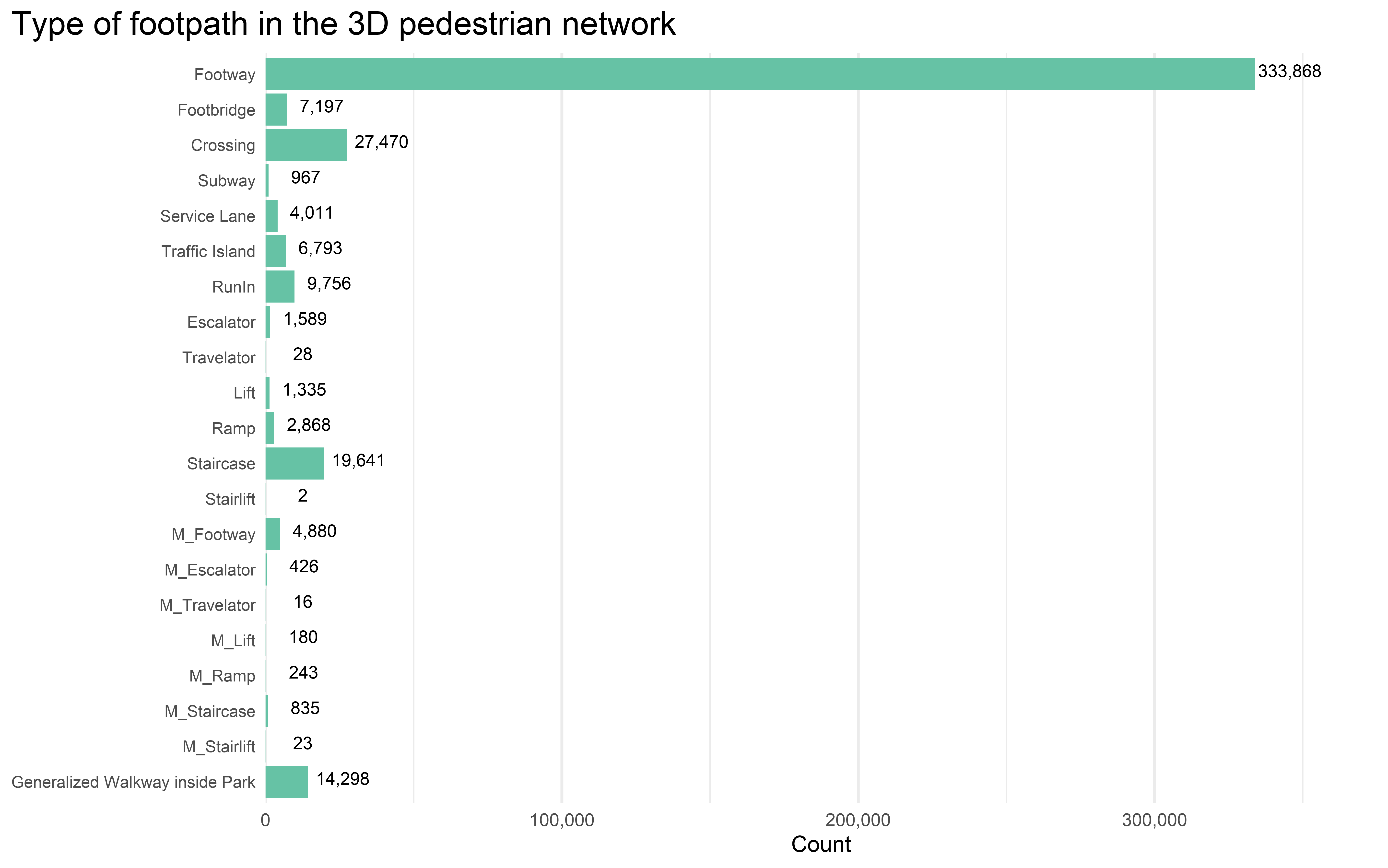
Types of footpath
Let’s dive into the dataset and take a glance in terms of summary statistics.
The level of details of the network already dropped my jaw - it has a total of 436426 path segments! An extremely large spatial dataset which contains only footpaths. About 334,000 paths are ubiquitous footway (i.e. sidewalk or pedestrian walkway). What also surprised me is that there are in total 27,470 crossings in the dataset. Although crossings are usually separated into two parts in the network sense (they are separated by the traffic islands), the total number of crossings still largely exceeds my random guess. Meanwhile, the 2,000 footbridges consist of 7,200 segments, and the 400 subways are split into about 1,000 segments.
PexNetwork_summary = PexNetwork_AttrTable %>%
  group_by(FeatureType) %>%
  summarise(
    count = n(),
    total_length = sum(SHAPE_Length),
    mean_length = mean(SHAPE_Length),
    median_length = median(SHAPE_Length)
  ) %>%
  merge(FeatureType_dict, by.x = "FeatureType", by.y = "Code")
ggplot(PexNetwork_summary, aes(y = reorder(DataType, desc(FeatureType)))) +
  geom_bar(aes(weight = count), fill = "#66c2a5") +
  # geom_text(stat = 'count', aes(label = count), hjust = 0) +
  geom_text(
    aes(y = DataType, x = count + 1000, label = format(count, big.mark=",")),
    hjust = 0,
    size = 3,
    # Not sure why need to nudge a little bit upward for the text
    nudge_y = .1,
    inherit.aes = TRUE
  ) +
  scale_x_continuous(labels = comma, limits = c(0,3.75e5), expand = c(0, 0)) +
  theme_bw() +
  theme(
    plot.title.position = "plot",
    plot.title = element_text(size = 16),
    panel.grid.major.y = element_blank(),
    panel.border = element_blank(),
    axis.text.y = element_text(size = 8),
    axis.title.y = element_blank(),
    axis.ticks = element_blank()
  ) +
  labs(
    title = "Type of footpath in the 3D pedestrian network",
    x = "Count"
  )
Distribution of path length
How about their distribution in terms of length and gradients?
Here I use the ggridges to visualise the shape of the distribution and relative height across each footpath type. I excluded the lifts category as their gradient and length are not useful at all - they are just some vertical lines and you will not “walk” on them.
In addition to the distribution, showing some critical values would allow those math nerds to grasp the look of the distribution quickly. Therefore, I also computed the median and mean value of each group.
As a supplementary note, the median and average length of all footpaths (excluding lifts category) are 8 m and 19 m respectively.
exclude_type = c("Lift", "Stairlift", "M_Lift", "M_Stairlift")

PexNetwork_AttrTable_typename = merge(PexNetwork_AttrTable, FeatureType_dict, by.x = "FeatureType", by.y = "Code") %>%
  filter(!(DataType %in% exclude_type))

PexNetwork_group_stat = PexNetwork_AttrTable_typename %>%
  filter(!(DataType %in% exclude_type)) %>%
  group_by(DataType, FeatureType) %>%
  summarise(
    group_mean_length = mean(SHAPE_Length),
    group_median_length = median(SHAPE_Length),
    group_mean_gradient = mean(Gradient),
    group_median_gradient = median(Gradient)
  )
MAX_PATH_LENGTH = 100
LENGTH_COLOUR = "#33A6B8"

# https://www.r-graph-gallery.com/301-custom-lollipop-chart.html
# https://cran.r-project.org/web/packages/ggridges/vignettes/introduction.html

ggplot(PexNetwork_AttrTable_typename, aes(x = SHAPE_Length, y = reorder(DataType, desc(FeatureType)))) +
  # lolipop-like base
  geom_segment(data = PexNetwork_group_stat,
               aes(x = 0, xend = group_median_length,
                   y = reorder(DataType, desc(FeatureType)), yend = reorder(DataType, desc(FeatureType))),
               colour = "#33A6B899", size = .75) +
  geom_segment(data = PexNetwork_group_stat,
               aes(x = group_median_length, xend = MAX_PATH_LENGTH,
                   y = reorder(DataType, desc(FeatureType)), yend = reorder(DataType, desc(FeatureType))),
               colour = "grey80", size = .75) +
  # ridges
  # position_nudge to move the ridge a little bit upwards to show lollipop
  geom_density_ridges(scale = 1.75, rel_min_height = 0.01, color = "#FFFFFF44", fill = "#33A6B899",
                               position = position_nudge(y = .11)) +
  # point for mean
  geom_point(data = PexNetwork_group_stat,
             aes(x = group_mean_length), shape = 21, size = 2, colour = LENGTH_COLOUR, fill = "#FFFFFF") +
  # point for median
  geom_point(data = PexNetwork_group_stat,
             aes(x = group_median_length), shape = 23, size = 2, colour = "grey20", fill = LENGTH_COLOUR, stroke = .5) +
  # indicate median value of each group
  geom_text(data = PexNetwork_group_stat,
    aes(y = DataType, x = group_median_length + 1, label = round(group_median_length, 2)),
    hjust = 0,
    size = 3,
    nudge_y = -.3,
    colour = LENGTH_COLOUR,
    fontface = "bold"
  ) +
  scale_x_continuous(limits = c(0, MAX_PATH_LENGTH)) +
  coord_cartesian(clip = "off") +
  theme_minimal() +
  theme(
    plot.title.position = "plot",
    plot.title = element_text(size = 16),
    panel.grid.minor.x = element_blank(),
    legend.position = "None",
    axis.title.y = element_blank(),
  ) +
  labs(
    title = "Distribution of path length, by feature type",
    subtitle = "Rhombus indicates the median and circle indicates the mean",
    x = "Path Length (m)",
    caption = "Note: Paths longer than 100m are not shown."
  )
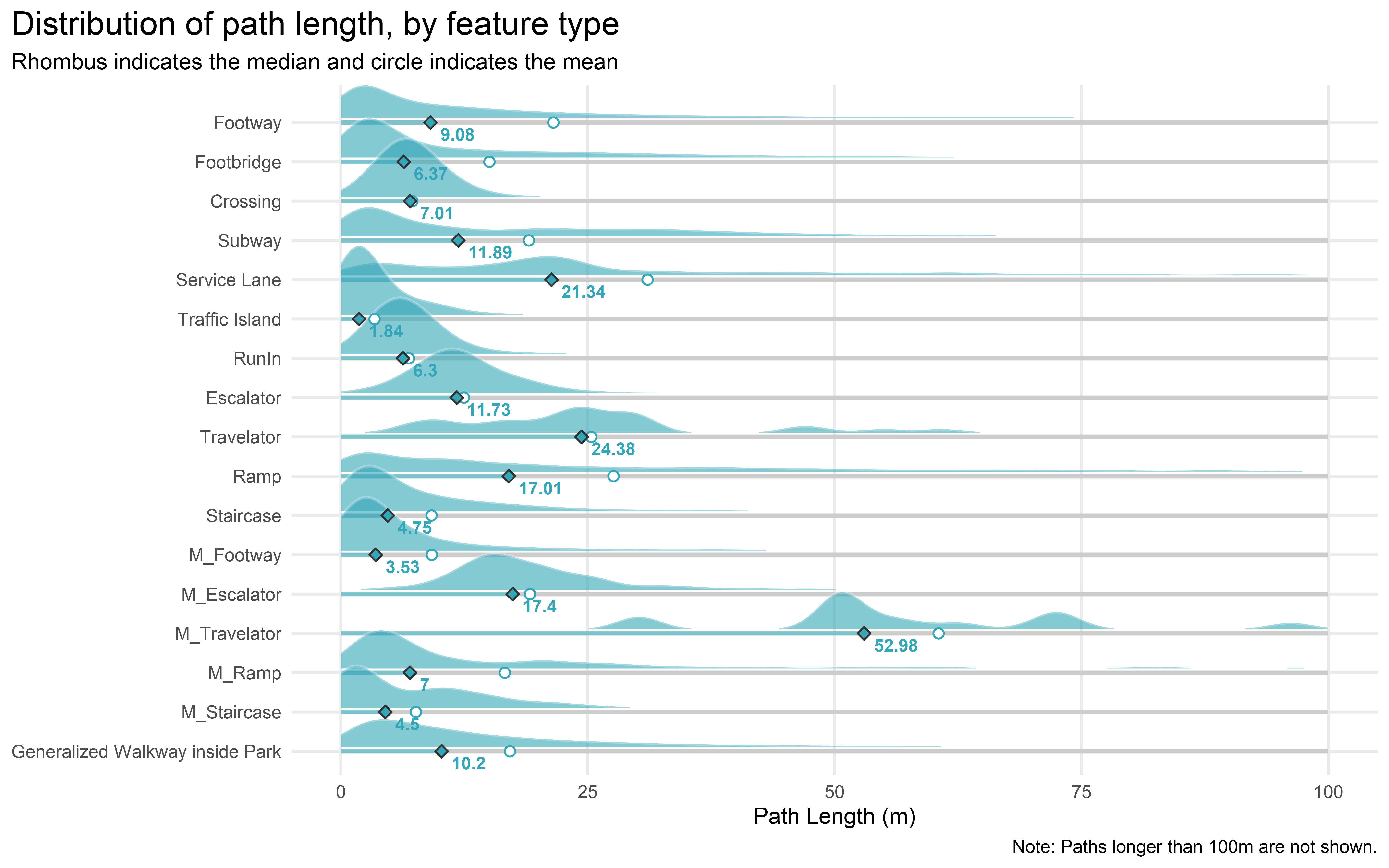
Travelator in MTR stations has the largest mean and median length. Not surprising when you consider the length of the travelators in HKU MTR Station, specifically those from the concourse to Exit C. Other long travelators include the one from Three Pacific Place to Admiralty Station.
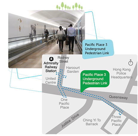 Photo Source: https://www.undergroundspace.gov.hk/pacificplace.htm
Distribution of path gradient
How about gradient? Again, as a supplementary note, the median and average gradient of all footpaths (excluding lifts category) are 0.01 and 0.06 respectively.
GRADIENT_COLOUR = "#ff7f00"
MAX_PATH_GRADIENT = 1

# https://www.r-graph-gallery.com/301-custom-lollipop-chart.html
# https://cran.r-project.org/web/packages/ggridges/vignettes/introduction.html

ggplot(PexNetwork_AttrTable_typename, aes(x = Gradient, y = reorder(DataType, desc(FeatureType)))) +
  # lolipop-like base
  geom_segment(data = PexNetwork_group_stat,
               aes(x = 0, xend = group_median_gradient,
                   y = reorder(DataType, desc(FeatureType)), yend = reorder(DataType, desc(FeatureType))),
               colour = "#ff7f0099", size = .75) +
  geom_segment(data = PexNetwork_group_stat,
               aes(x = group_median_gradient, xend = MAX_PATH_GRADIENT,
                   y = reorder(DataType, desc(FeatureType)), yend = reorder(DataType, desc(FeatureType))),
               colour = "grey80", size = .75) +
  # ridges
  # position_nudge to move the ridge a little bit upwards to show lollipop
  geom_density_ridges(scale = 1.25, rel_min_height = 0.01, color = "#FFFFFF44", fill = "#ff7f0099",
                               position = position_nudge(y = .11)) +
  # point for mean
  geom_point(data = PexNetwork_group_stat,
             aes(x = group_mean_gradient), shape = 21, size = 2, colour = GRADIENT_COLOUR, fill = "#FFFFFF") +
  # point for median
  geom_point(data = PexNetwork_group_stat,
             aes(x = group_median_gradient), shape = 23, size = 2, colour = "grey20", fill = GRADIENT_COLOUR, stroke = .5) +
  # indicate median value of each group
  geom_text(data = PexNetwork_group_stat,
    aes(y = DataType, x = group_median_gradient + .01, label = round(group_median_gradient, 3)),
    hjust = 0,
    size = 3,
    nudge_y = -.3,
    colour = GRADIENT_COLOUR,
    fontface = "bold"
  ) +
  scale_x_continuous(limits = c(0, MAX_PATH_GRADIENT)) +
  coord_cartesian(clip = "off") +
  theme_minimal() +
  theme(
    plot.title.position = "plot",
    plot.title = element_text(size = 16),
    panel.grid.minor.x = element_blank(),
    legend.position = "None",
    axis.title.y = element_blank(),
  ) +
  labs(
    title = "Distribution of path graident, by feature type",
    subtitle = "Rhombus indicates the median and circle indicates the mean",
    x = "Gradient",
    caption = "Note: Paths with gradient larger than 1 are not shown."
  )
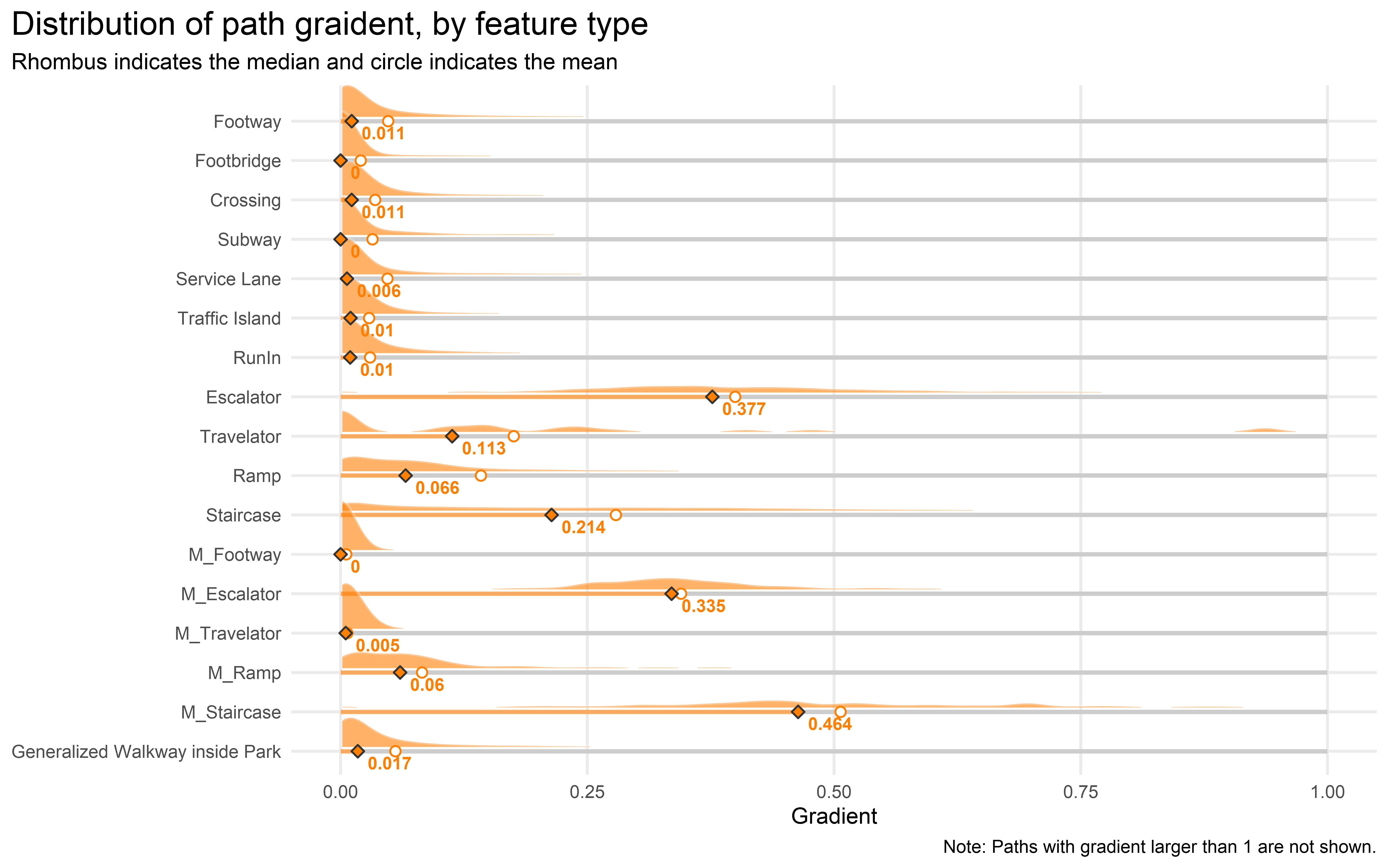
One interesting observation is that the gradient of the staircases (i.e. steepness of the stairs) in MTR stations is much higher than the normal staircases.
Gradient of normal footpaths on ground level has median around 0.01 to 0.02, while the mean is around 0.04 to 0.06. We can see the distribution of gradient is positively skewed. Again, this is not surprising as the footpaths in the main area of the city are mostly built on flatland. However, there are abundant steep footpaths located in the hilly districts like Sai Ying Pun and Tsz Wan Shan.
It could be something worth investigating by classifying the footpaths by residential areas, then investigate the differences of slopes across various districts. A “Steepness Index” of each residential area could be computed. The steepness of the path could be used as an indicator to measure walkability. We could even look into the correlation between this index and flat price!
Hiatus
This blog is just a quick review of the properties of the pedestrian network. The power and possible usage of the network dataset are unimaginable, especially for accessibility analysis. The best way to understand the dataset is to play the juggle the dataset around, looking into the shapes and attributes. If you are interested in investigating pedestrian walking behaviour, this dataset is a gold mine for you to explore.